And wits were matched.

Your R Club buddies have been experimenting with ways to plot data with ggplot. Below is a sampling of their efforts. Your duty this week was to choose at least three plots and figure out how they were plotted.

Getting ready

We’ll start by reading in the Tomato Dataset and getting rid of NA values.

tomato <- read.table("TomatoR2CSHL.csv", header = T, sep = ",")
tomato <- na.omit(tomato)
library(ggplot2)

In addition to the Tomato Dataset that we’ve been using, people have made plots with the movies and mpg datasets (which come with ggplot2 and are, therefore, loaded with library(ggplot2)). If the datasets don’t look familiar, be sure to scroll down to the ‘Data’ section of the ggplot2 docs.

Approach to solving challenges

When trying to figure out how to write the code for a plot, I recommend making a quick set of observations:

For many plots, you can take this information and plug it into some ggplot functions to get a decent first draft. Next you are ready to make a couple more observations to make further improvements:

• Are any custom color, size, etc. scales being used? If so, is the relevant data discrete or continuous?
• Have labels been customized?

Taken together, these observations essentially serve as pseudocode for the plot in question.

Challenge 1

Stacey used the movies dataset to plot movie rating since the dawn of cinematography (binned by density) .

Figure 1A:

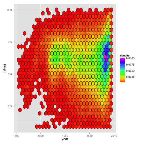
Based on our observations, we see that Figure 1A uses geom_hex() (which bins a 2-dimensional plane into hexagons) to plot movie rating by year. By default, the hexagons are colored based on the number of counts in each hexagon; however, Stacey manually set the fill = ..density.. when she made her plot:

ggplot(movies) +
  geom_hex(aes(x    = year,
               y    = rating,
               fill = ..density..),
           color = "black") +
  scale_fill_gradientn(colours = rainbow(7))

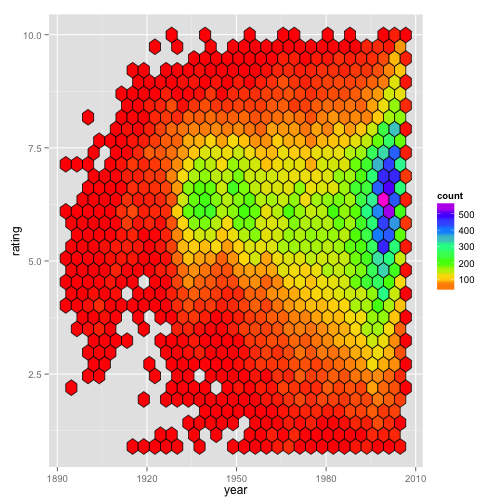
In this case, the only real difference between counts and density is seen with the scale bar in the legend. Below (Fig. 1B) is the same plot, but with the default fill (i.e., counts) being used. The graphical regions of the plot Figures 1A and 1B are identical.

Figure 1B:

ggplot(movies) +
  geom_hex(aes(x = year,
               y = rating),
           color = "black") +
  scale_fill_gradientn(colours = rainbow(7))

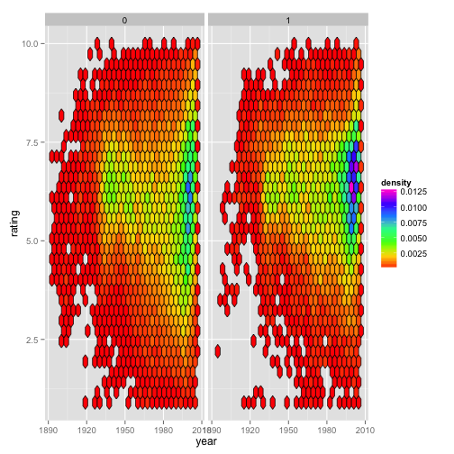
However, if we were to instead make this plot faceted, we begin to see the difference between the ‘counts’ and ‘density’. The next two figures are faceted by whether the movie being considered is a drama. The first one shows that with the default method, the fill color is scaled relative to all the data for the entire plot (Fig. 1C), whereas mapping fill = ..density.. results in the data within each panel being scaled relative to the relevant panel (Fig. 1D).

Figure 1C:

ggplot(movies) +
  geom_hex(aes(x = year,
               y = rating),
           color = "black") +
  scale_fill_gradientn(colours = rainbow(7)) +
  facet_grid(. ~ Drama)

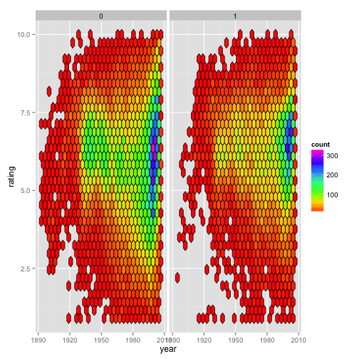
Figure 1D:

ggplot(movies) +
  geom_hex(aes(x    = year,
               y    = rating,
               fill = ..density..),
           color = "black") +
  scale_fill_gradientn(colours = rainbow(7)) +
  facet_grid(. ~ Drama)

When reproducing this plot, many people had issues with setting the border of each hexbin to black. To set the color successfully, you need to remember two things:

• The color of lines, dots, borders, etc. is specified with color and the fill color for shapes with fill.
• When you are mapping an aesthetic to a variable (of your dataset), you specify that inside aes(); however, when setting an aesthetic to a constant value, color, etc., it needs to be done outside of aes(). I’ve formatted the indentation pattern of the code snippets above to reinforce the fact that x, y, and, fill are aesthetics, but color is not.

Challenge 2

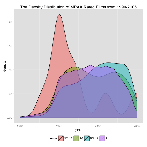
Ciera plotted MPAA movie rating trends over the last couple decades.

Figure 2:

We need to start by sub-setting the movies such that we are only considering movies with MPAA ratings since 1990. Here are two equally valid ways to subset the data:

movies.mpaa.new <- subset(movies, mpaa != "" & year >= 1990)

movies.mpaa.new <- movies[movies$mpaa != "" & movies$year >= 1990, ]

There are multiple ways to assemble the code for building a plot. To emphasize the different layers/components of a ggplot2-generated figure, we’ll assign each part of the plot to a separate variable and then combine them to generate Figure 2.

For the base of the plot, we specify the data subset (movies.mpaa.new) that we just created and map the aesthetics x and fill. Unlike geom_hex() plots, color in a geom_density() plot defaults to black so we don’t need to set it.

base <- ggplot(movies.mpaa.new,
               aes(x    = year,
                   fill = mpaa))

Next, we specify the geom_density() layer. In order to see the densities for each MPAA rating, we need to change alpha (the transparency setting). For her plot, Ciera set alpha = 1/2. Note that it is not inside aes(), because we are setting it to an absolute value rather than mapping it to a data attribute. Also, we must place it inside geom_density(), not ggplot(). Typically, you only specify the dataset and aesthetics with ggplot().

density <- geom_density(alpha = 1/2)

Using labs(), we can customize the labels for the entire plot, the axes, and/or the legend scales.

label <- labs(title = "The Density Distribution of MPAA Rated Films from 1990-2005")

To move the legend from the right-side of the figure to the bottom, we can set the legend.position element with theme().

theme.custom <- theme(legend.position = "bottom")

Now that we’ve defined each component of Figure 2, we can put them together like this:

base + density + label + theme.custom

I won’t bother actually plotting this here, because it will be identical to Figure 2; however, I hope you can see the potential here for highly-readable modular customization. Rather than copy and pasting a big chunk of code for making small changes to create new plots, you can assign to variables any parts that you want to remain constant between your plots.

Challenge 3

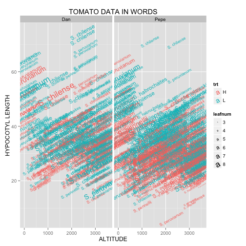
Miguel is a huge fan of the written word. One of his life goals is to bridge the gap between science and literature. He made this plot in hopes of advancing this cause.

Figure 3A:

Figure 3A can be generated with:

ggplot(tomato, aes(x     = alt,
                   y     = hyp,
                   size  = leafnum,
                   label = species,
                   color = trt,
                   angle = 30)) +
  geom_text() +
  facet_grid(. ~ who) +
  labs(title = "TOMATO DATA IN WORDS",
       x     = "ALTITUDE",
       y     = "HYPOCOTYL LENGTH")

Here, we see geom_text() in action. As usual, we start by specifying the dataset and aesthetics within ggplot(). If you look closely, you’ll notice that angle is the exception to the rule regarding mapping vs. setting. Even though we are setting angle = 30 rather than mapping it to a parameter from the dataset, it must be placed inside aes(). Putting it in what should be the proper place (geom_text(angle = 30)), causes the words to be plotted at a 30° angle, but also results in the letters in the legend to be angled as shown in Figure 3B.

Figure 3B:

ggplot(tomato, aes(x     = alt,
                   y     = hyp,
                   size  = leafnum,
                   label = species,
                   color = trt)) +
  geom_text(angle = 30) +
  facet_grid(. ~ who) +
  labs(title = "TOMATO DATA IN WORDS",
       x     = "ALTITUDE",
       y     = "HYPOCOTYL LENGTH")

I think either approach is reasonable, but the legend in Figure 3A looks a bit more clean to me. As for the other parts of the code, note how labs() is used to specify labels for the entire plot and both axes. A less elegant, yet completely functional alternative approach is:

+ ggtitle("TOMATO DATA IN WORDS") +
  xlab("ALTITUDE") +
  ylab("HYPOCOTYL LENGTH")

Challenge 4

Cody found a geom that can be used to compare distributions by plotting them along the axes. Can you find it, too?

Figure 4:

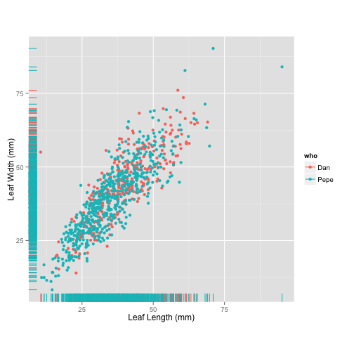
ggplot(tomato, aes(x      = leafleng,
                   y      = leafwid,
                   colour = who)) +
    geom_point() +
    geom_rug() +
    labs(x = "Leaf Length (mm)",
         y = "Leaf Width (mm)") +
    theme(aspect.ratio = 1)

Challenge 5

For Valentine’s Day, Jessica received a $20 gift card for a local gas station. Before she redeems it, she wants to find out which types of car will get her to the Bay Area and back on five gallons.

Figure 5:

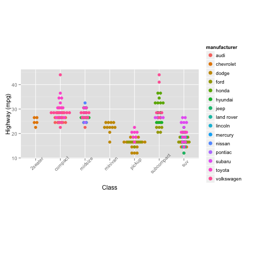
ggplot(mpg, aes(x      = class,
                y      = hwy,
                colour = manufacturer,
                fill   = manufacturer)) +
  geom_dotplot(binaxis      = "y",
               stackdir     = "center",
               binpositions = "all") +
  labs (x = "Class",
        y = "Highway (mpg)") +
  theme(aspect.ratio = 0.5,
        axis.text.x  = element_text(angle = 45))

Challenge 6

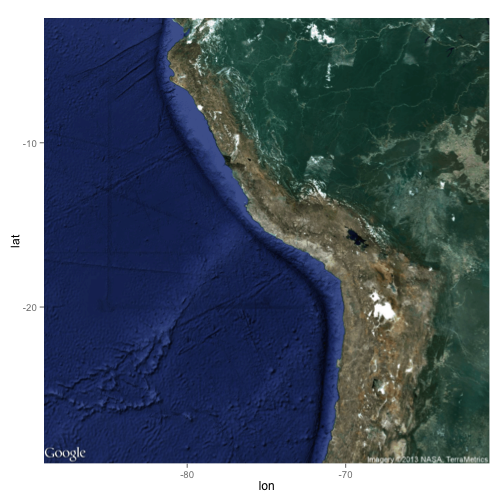
Hsin-Yen was curious about the terrain and altitude where various tomato species have been found in the wild.

Figure 6A:

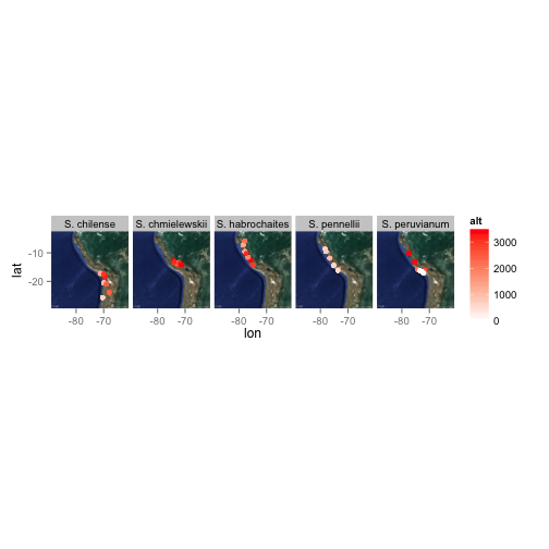
Figure 6B:

ggmap(map)

ggmap(map) +
  geom_point(aes(x      = lon,
                 y      = lat,
                 colour = alt),
             data = tomato,
             size = 2) +
  facet_grid(. ~ species) +
  scale_colour_continuous(low  = "white",
                          high = "red")

Challenge 7

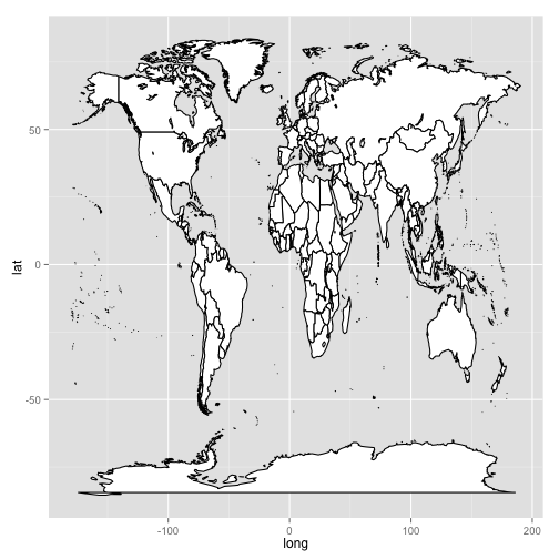
Not one to be outdone, Stacey demonstrates that she also knows the ways of the world by plotting the geographical position of tomato species collection points on top of not just a part of South America, but on top of the entire world.

Figure 7A:

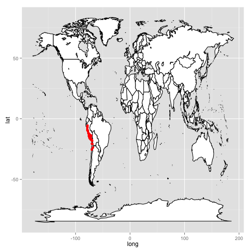
Figure 7B:

world <- map_data("world")
worldmap <- ggplot(world, aes(x     = long,
                              y     = lat,
                              group = group)) +
  geom_polygon(fill   = "white",
               colour = "black")
worldmap

worldmap +
  geom_point(aes(x     = lon,
                 y     = lat,
                 group = NULL),
             data  = tomato,
             size  = 2,
             color = "red")