R Homework for April 4, 2013
Section 1: Data Types
Questions 1 to 6 refer to the file ELF3s_bolting_Rclub.csv. Import it now.
Q1
What data types are represented in each column?
data <- read.csv("~/Documents/Teaching/RClub/webSite/downloads/ELF3s_bolting_Rclub.csv")

# one way is to do a summary and figure it out from the way the output is
# formatted
summary(data)
##        Plant        diameter      n_leaves    flowering_time treatment
##  Sh2.H4.1h:  2   33.99  :  3   Min.   : 0.0   Min.   :18.0   h:207
##  Ba1.A1.1h:  1   29.43  :  2   1st Qu.: 7.0   1st Qu.:23.0   l:208
##  Ba1.A1.1l:  1   30.84  :  2   Median : 8.0   Median :27.0
##  Ba1.A1.3h:  1   32.52  :  2   Mean   :10.3   Mean   :29.6
##  Ba1.A1.3l:  1   33.43  :  2   3rd Qu.:13.0   3rd Qu.:36.0
##  Ba1.A1.5h:  1   33.73  :  2   Max.   :52.0   Max.   :53.0
##  (Other)  :408   (Other):402
##  genotype  transformation      flat           col           row
##  Bay:204   Ba1:138        Min.   : 1.0   H      : 49   Min.   :1.00
##  Sha:211   Ba3: 66        1st Qu.: 3.5   A      : 48   1st Qu.:1.00
##            Sh1: 70        Median : 6.0   B      : 48   Median :2.00
##            Sh2: 71        Mean   : 6.5   G      : 48   Mean   :2.46
##            Sh3: 70        3rd Qu.:10.0   D      : 47   3rd Qu.:3.00
##                           Max.   :12.0   E      : 47   Max.   :4.00
##                                          (Other):128
# factor: Plant, diameter, treatment, genotype, transformation, col,
# numeric: n_leaves, flowering_time, flat, row

# alternative:
str(data)
## 'data.frame':	415 obs. of  10 variables:
##  $ Plant         : Factor w/ 414 levels "Ba1.A1.1h","Ba1.A1.1l",..: 159 155 35 215 257 377 347 285 291 88 ...
##  $ diameter      : Factor w/ 392 levels "0","21.54","21.62",..: 134 272 101 187 218 225 254 152 244 182 ...
##  $ n_leaves      : int  7 8 7 7 7 7 10 9 10 9 ...
##  $ flowering_time: int  23 22 27 25 25 29 28 28 29 28 ...
##  $ treatment     : Factor w/ 2 levels "h","l": 1 1 1 1 1 1 1 1 1 1 ...
##  $ genotype      : Factor w/ 2 levels "Bay","Sha": 1 1 1 2 2 2 2 2 2 1 ...
##  $ transformation: Factor w/ 5 levels "Ba1","Ba3","Sh1",..: 2 2 1 3 3 5 5 4 4 1 ...
##  $ flat          : int  1 1 1 1 1 1 1 1 1 1 ...
##  $ col           : Factor w/ 9 levels "A","B","C","D",..: 3 3 2 2 7 5 1 3 4 6 ...
##  $ row           : int  3 2 4 3 1 2 2 4 3 1 ...
Q2
a) Are there any columns that you think have the wrong data type?
Yes
b) Which ones? see below
c) Why?
Diameter should be numeric because we would want to analyze the actual measurements. Flat and row should be factor becuase these are used to group plants.
Q3
How would you change the columns to their correct types?
# For row and flat:
data$flat <- as.factor(data$flat)
data$row <- as.factor(data$row)

# It isn't so simple for diameter. First is to determine why diameter came
# in as a factor instead of numeric. There must be a non-numeric value
# somewhere in there and we need to find it.

# can we just use as.numeric?
as.numeric(data$diameter)
##   [1] 134 272 101 187 218 225 254 152 244 182 275 194 245 309 162 178 205
##  [18] 284 297 288 362 356 303 327 350 348 373 383 378 311 385 359 377 375
##  [35] 377 386 173 149  81 220 156  47 106  68 233 136 229 212 154 224 216
##  [52] 144  58 179 237 210   1 104 137  93  54 266 272 238 184 262 171 278
##  [69] 202 189 230 226  69 236 192 279 265 215 260 291 302 238 190  95 213
##  [86] 289 287 347 352 277 295 274 310 371 294 313 345 335 118 319 382 388
## [103] 365 164  74 112  21  29  62   5 183  53 103 105  70  78  45  82  23
## [120]  87 227 198 181  51  41 143  72 204  91  55  61 252 169 283 222  25
## [137] 242  71 231  59 188 135 200 260 182 264 250  52 263 138 159 281 276
## [154] 304 337 356 296 308 333 351 305 332 344 338 361 341 369 357 346 330
## [171] 381 392 292  39  13  14 126  90   2  38  67  85 121  40  10  30  54
## [188]  86 119  64  36  57  56 158 155  73  96 133 151 130 193 191 110 163
## [205] 108 146 234   4 122  66 123  80 168 129 175 177 219  79 184 282 251
## [222] 268 286 301 306 318 317 322 334 307 329 344 354 340 349 326 328 321
## [239] 331 364 387 384  22  32  65   3   8  24  11  43  67  26   9  17  94
## [256]  44  18 107 102 127  34  63 151 185  28 120  20 113 125 203 165 115
## [273] 222 148 132 293 124 128 116  75  60  48  97  83 247 239 139 243 228
## [290] 186 249 206 314 267 257 353 312 299 372 343 323 320 342 355 380 363
## [307] 368 379 389 391  16  33  12  46   6  50  31  37  15  27   7  19 176
## [324] 117 111 141 109  76 160  98 113  99 180 113 261 197 174  92 258  90
## [341] 172 253 232 270 300 140 114 100 211 131 214 145 142 167 259 298 201
## [358] 271 241 240 296 147  84 325 316 285 239 339 336 324 315 273 370 366
## [375] 367 358 360 376 374 390  77  42  35 161  88  49 150 153 196 166 207
## [392] 246 157 195 221 199 217  89 170 248 231 102 233 256 235 236 237 209
## [409] 255 107 269 208 280 223 290
# No! this returns the integer representation of the factor levels.

# instead:
as.numeric(as.character(data$diameter))
## Warning: NAs introduced by coercion
##   [1] 35.40 49.68 33.42 39.41 42.14 42.93 46.64 36.45 45.11 38.96 50.10
##  [12] 39.79 45.18 55.69 37.35 38.66 40.72 50.88 53.78 51.40 71.47 69.36
##  [23] 54.49 60.81 66.73 66.18 74.57 80.54 77.97 56.39 82.37 70.70 77.02
##  [34] 75.00 77.02 82.54 38.35 36.30 31.69 42.21 36.60 28.29 33.65 30.90
##  [45] 43.84 35.53 43.38 41.39 36.48 42.81 41.98 35.98 29.90 38.70 44.10
##  [56] 41.03  0.00 33.47 35.66 32.69 29.43 47.97 49.68 44.20 39.04 47.34
##  [67] 38.10 50.28 40.46 39.54 43.40    NA 30.96 44.05 39.67 50.30 47.92
##  [78] 41.84 47.14 51.88 54.46 44.20 39.61 32.95 41.55 51.41 51.11 65.83
##  [89] 67.31 50.18 53.36 50.02 56.19 73.70 52.42 56.45 65.10 63.49 34.16
## [100] 58.42 80.48 83.49 71.68 37.45 31.19 33.98 25.92 26.63 30.35 22.40
## [111] 38.98 29.34 33.45 33.54 31.05 31.42 27.83 31.77 26.20 32.30 43.11
## [122] 40.12 38.92 28.69 27.66 35.97 31.09 40.63 32.53 29.57 30.07 46.55
## [133] 38.00 50.74 42.25 26.25 45.02 31.06 43.45 29.99 39.52 35.48 40.37
## [144] 47.14 38.96 47.85 46.16 28.82 47.39 35.69 37.12 50.63 50.16 54.71
## [155] 64.31 69.36 53.44 55.66 62.93 67.12 54.78 62.32 64.86 64.60 71.16
## [166] 64.75 72.76 70.27 65.75 61.52 80.30 89.98 51.97 27.45 24.13 24.17
## [177] 34.59 32.52 21.54 27.44 30.84 31.92 34.22 27.53 23.63 27.02 29.43
## [188] 31.99 34.17 30.62 27.23 29.77 29.70 37.03 36.59 31.12 33.00 35.25
## [199] 36.36 34.86 39.77 39.63 33.93 37.41 33.85 36.02 43.90 22.20 34.27
## [210] 30.83 34.35 31.59 37.92 34.84 38.44 38.59 42.16 31.49 39.04 50.70
## [221] 46.27 48.69 51.04 54.40 55.12 58.38 57.80 59.22 63.27 55.20 61.05
## [232] 64.86 67.68 64.69 66.20 59.93 60.95 58.82 62.31 71.52 82.64 80.86
## [243] 26.11 27.11 30.78 21.62 23.38 26.21 23.81 27.70 30.84 26.34 23.57
## [254] 25.31 32.72 27.79 25.36 33.73 33.43 34.64 27.21 30.38 36.36 39.20
## [265] 26.53 34.21 25.57 33.99 34.48 40.57 37.59 34.08 42.25 36.25 35.12
## [276] 52.30 34.37 34.70 34.09 31.33 30.04 28.33 33.01 31.81 45.57 44.41
## [287] 35.81 45.07 43.36 39.35 45.94 40.79 56.78 48.25 46.94 67.34 56.40
## [298] 54.08 74.52 64.85 59.30 58.74 64.79 67.73 79.72 71.49 72.53 79.02
## [309] 85.71 89.73 24.60 27.13 23.89 28.18 23.00 28.57 27.05 27.41 24.42
## [320] 26.49 23.30 25.51 38.52 34.10 33.97 35.94 33.87 31.40 37.18 33.33
## [331] 33.99 33.39 38.79 33.99 47.25 40.08 38.40 32.63 47.11 32.52 38.11
## [342] 46.60 43.51 49.30 54.22 35.92 34.07 33.41 41.26 35.09 41.77 36.00
## [353] 35.96 37.87 47.13 53.91 40.40 49.65 44.95 44.62 53.44 36.15 31.87
## [364] 59.77 57.68 50.92 44.41 64.64 63.57 59.53 56.99 50.01 73.69 72.09
## [375] 72.21 70.38 70.74 75.14 74.66 88.73 31.41 27.69 27.22 37.30 32.35
## [386] 28.52 36.33 36.47 39.99 37.85 40.88 45.40 36.90 39.81 42.24 40.20
## [397] 42.01 32.47 38.02 45.88 43.45 33.43 43.84 46.93 44.02 44.05 44.10
## [408] 40.98 46.68 33.73 49.17 40.90 50.45 42.59 51.47
# or:
as.numeric(levels(data$diameter)[data$diameter])
## Warning: NAs introduced by coercion
##   [1] 35.40 49.68 33.42 39.41 42.14 42.93 46.64 36.45 45.11 38.96 50.10
##  [12] 39.79 45.18 55.69 37.35 38.66 40.72 50.88 53.78 51.40 71.47 69.36
##  [23] 54.49 60.81 66.73 66.18 74.57 80.54 77.97 56.39 82.37 70.70 77.02
##  [34] 75.00 77.02 82.54 38.35 36.30 31.69 42.21 36.60 28.29 33.65 30.90
##  [45] 43.84 35.53 43.38 41.39 36.48 42.81 41.98 35.98 29.90 38.70 44.10
##  [56] 41.03  0.00 33.47 35.66 32.69 29.43 47.97 49.68 44.20 39.04 47.34
##  [67] 38.10 50.28 40.46 39.54 43.40    NA 30.96 44.05 39.67 50.30 47.92
##  [78] 41.84 47.14 51.88 54.46 44.20 39.61 32.95 41.55 51.41 51.11 65.83
##  [89] 67.31 50.18 53.36 50.02 56.19 73.70 52.42 56.45 65.10 63.49 34.16
## [100] 58.42 80.48 83.49 71.68 37.45 31.19 33.98 25.92 26.63 30.35 22.40
## [111] 38.98 29.34 33.45 33.54 31.05 31.42 27.83 31.77 26.20 32.30 43.11
## [122] 40.12 38.92 28.69 27.66 35.97 31.09 40.63 32.53 29.57 30.07 46.55
## [133] 38.00 50.74 42.25 26.25 45.02 31.06 43.45 29.99 39.52 35.48 40.37
## [144] 47.14 38.96 47.85 46.16 28.82 47.39 35.69 37.12 50.63 50.16 54.71
## [155] 64.31 69.36 53.44 55.66 62.93 67.12 54.78 62.32 64.86 64.60 71.16
## [166] 64.75 72.76 70.27 65.75 61.52 80.30 89.98 51.97 27.45 24.13 24.17
## [177] 34.59 32.52 21.54 27.44 30.84 31.92 34.22 27.53 23.63 27.02 29.43
## [188] 31.99 34.17 30.62 27.23 29.77 29.70 37.03 36.59 31.12 33.00 35.25
## [199] 36.36 34.86 39.77 39.63 33.93 37.41 33.85 36.02 43.90 22.20 34.27
## [210] 30.83 34.35 31.59 37.92 34.84 38.44 38.59 42.16 31.49 39.04 50.70
## [221] 46.27 48.69 51.04 54.40 55.12 58.38 57.80 59.22 63.27 55.20 61.05
## [232] 64.86 67.68 64.69 66.20 59.93 60.95 58.82 62.31 71.52 82.64 80.86
## [243] 26.11 27.11 30.78 21.62 23.38 26.21 23.81 27.70 30.84 26.34 23.57
## [254] 25.31 32.72 27.79 25.36 33.73 33.43 34.64 27.21 30.38 36.36 39.20
## [265] 26.53 34.21 25.57 33.99 34.48 40.57 37.59 34.08 42.25 36.25 35.12
## [276] 52.30 34.37 34.70 34.09 31.33 30.04 28.33 33.01 31.81 45.57 44.41
## [287] 35.81 45.07 43.36 39.35 45.94 40.79 56.78 48.25 46.94 67.34 56.40
## [298] 54.08 74.52 64.85 59.30 58.74 64.79 67.73 79.72 71.49 72.53 79.02
## [309] 85.71 89.73 24.60 27.13 23.89 28.18 23.00 28.57 27.05 27.41 24.42
## [320] 26.49 23.30 25.51 38.52 34.10 33.97 35.94 33.87 31.40 37.18 33.33
## [331] 33.99 33.39 38.79 33.99 47.25 40.08 38.40 32.63 47.11 32.52 38.11
## [342] 46.60 43.51 49.30 54.22 35.92 34.07 33.41 41.26 35.09 41.77 36.00
## [353] 35.96 37.87 47.13 53.91 40.40 49.65 44.95 44.62 53.44 36.15 31.87
## [364] 59.77 57.68 50.92 44.41 64.64 63.57 59.53 56.99 50.01 73.69 72.09
## [375] 72.21 70.38 70.74 75.14 74.66 88.73 31.41 27.69 27.22 37.30 32.35
## [386] 28.52 36.33 36.47 39.99 37.85 40.88 45.40 36.90 39.81 42.24 40.20
## [397] 42.01 32.47 38.02 45.88 43.45 33.43 43.84 46.93 44.02 44.05 44.10
## [408] 40.98 46.68 33.73 49.17 40.90 50.45 42.59 51.47
# The warning tells us that there was a problem in the conversion, this is
# probably our problem observation

# find it with:
data[is.na(as.numeric(as.character(data$diameter))), ]
## Warning: NAs introduced by coercion
##        Plant diameter n_leaves flowering_time treatment genotype
## 72 Ba1.G2.2h   43. 68       10             27         h      Bay
##    transformation flat col row
## 72            Ba1    3   G   2
# Aha an extra space!

# an alternative way to find this would be:
grep("[^0-9\\.]+", data$diameter, value = T)
## [1] "43. 68"
# which translates into find any item that contains something other than
# the digits 0-9 and a decimal point. We will have a session on grep at
# some later point.

# fix it with:
data$diameter <- as.character(data$diameter)
data$diameter[data$diameter == "43. 68"] <- 43.68
data$diameter <- as.numeric(data$diameter)

# or, more generally:
data$diameter <- as.numeric(sub(" ", "", data$diameter))
# this searches for a space and substitutes an empty string We don't have
# to convert to a character because sub does this automatically

# An alternative way to change data types in the data frame, from Aashish
data_mod <- transform(data, diameter = as.numeric(as.character(diameter)), flat = as.factor(flat),
    row = as.factor(row))
Q4
Are there any obvious mistakes in this data frame beyond what you might have found in answering Q3?
# quick check is with summary
summary(data)
##        Plant        diameter       n_leaves    flowering_time treatment
##  Sh2.H4.1h:  2   Min.   : 0.0   Min.   : 0.0   Min.   :18.0   h:207
##  Ba1.A1.1h:  1   1st Qu.:33.4   1st Qu.: 7.0   1st Qu.:23.0   l:208
##  Ba1.A1.1l:  1   Median :40.1   Median : 8.0   Median :27.0
##  Ba1.A1.3h:  1   Mean   :44.2   Mean   :10.3   Mean   :29.6
##  Ba1.A1.3l:  1   3rd Qu.:52.1   3rd Qu.:13.0   3rd Qu.:36.0
##  Ba1.A1.5h:  1   Max.   :90.0   Max.   :52.0   Max.   :53.0
##  (Other)  :408
##  genotype  transformation      flat          col      row
##  Bay:204   Ba1:138        1      : 36   H      : 49   1:107
##  Sha:211   Ba3: 66        4      : 35   A      : 48   2:106
##            Sh1: 70        6      : 35   B      : 48   3:106
##            Sh2: 71        10     : 35   G      : 48   4: 96
##            Sh3: 70        11     : 35   D      : 47
##                           12     : 35   E      : 47
##                           (Other):204   (Other):128
# Plants with diameter 0 and 0 leaves; seems unusual Also there are two
# entries for Sh2.H4.1h

# lets look at the duplicated entry a little more closely
data[duplicated(data$Plant), ]  #only shows us the second row
##        Plant diameter n_leaves flowering_time treatment genotype
## 35 Sh2.H4.1h    77.02       20             44         h      Sha
##    transformation flat col row
## 35            Sh2    1   H   4
dup.plant <- data$Plant[duplicated(data$Plant)]
data[data$Plant == dup.plant, ]
##        Plant diameter n_leaves flowering_time treatment genotype
## 33 Sh2.H4.1h    77.02       20             44         h      Sha
## 35 Sh2.H4.1h    77.02       20             44         h      Sha
##    transformation flat col row
## 33            Sh2    1   H   4
## 35            Sh2    1   H   4
# since the values are the same we can just remove it with:
data <- data[!duplicated(data$Plant), ]
# OR
data <- unique(data)

# what about the strange plants with zero diameter? might be worth doing a
# quick visual check of outliers:
library(reshape)
library(ggplot2)
melt.data <- melt(data, measure.vars = c("diameter", "n_leaves", "flowering_time"))
pl <- ggplot(melt.data, aes(x = variable, y = value))
pl + geom_jitter() + facet_wrap(~variable, scales = "free_y")
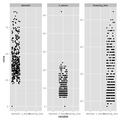
# flowering time and n_leaves of 0 seems odd.  n_leaves of 50 perhaps a
# bit strange lets look at these rows
data[data$diameter == 0, ]
##        Plant diameter n_leaves flowering_time treatment genotype
## 57 Ba1.B4.1l        0        0             23         l      Bay
##    transformation flat col row
## 57            Ba1    2   B   4
# remove row with 0 measurements
data <- data[data$diameter > 0, ]

# look at row with more than 50 leaces
data[data$n_leaves > 50, ]
##         Plant diameter n_leaves flowering_time treatment genotype
## 242 Ba1.H3.4h    80.86       52             53         h      Bay
##     transformation flat col row
## 242            Ba1    7   H   3
# also has among the largest diameters and latest flowering times, so
# seems real.
Q5
Make the “Sha” genotype the reference level for the genotype column
data$genotype <- relevel(data$genotype, ref = "Sha")
Q6
Change the order of levels in “trasformation” to be Sh1, Sh2, Sh3, Ba1, Ba3
data$genotype <- factor(data$genotype, levels = c("Sh1", "Sh2", "Sh3", "Ba1",
    "Ba3"))
Section 2: Reshape
The remaining questions deal with the reshape package and the tomato dataset.
- Read my post on reshape on the Rclub website
- Additional information on reshape is in section 9.2 of the ggplot book
- import the standard tomato data set.
tomato <- read.csv("~/Documents/Teaching/RClub/TomatoRClub.csv")
Q7
What are the id variables and measure variables in the Tomato data set?
head(tomato)
##   shelf flat col row    acs trt days   date   hyp int1 int2 int3 int4
## 1     Z    1   B   1 LA2580   H   28 5/5/08 19.46 2.37 1.59 1.87 0.51
## 2     Z    1   C   1 LA1305   H   28 5/5/08 31.28 3.34 0.01 9.19 1.62
## 3     Z    1   D   1 LA1973   H   28 5/5/08 56.65 8.43 2.39 6.70 3.69
## 4     Z    1   E   1 LA2748   H   28 5/5/08 35.18 0.56 0.00 1.60 0.61
## 5     Z    1   F   1 LA2931   H   28 5/5/08 35.32 0.82 0.02 1.49 0.46
## 6     Z    1   G   1 LA1317   H   28 5/5/08 28.74 1.07 6.69 5.72 4.76
##   intleng totleng petleng leafleng leafwid leafnum ndvi     lat    lon
## 1    6.34   25.80   15.78    30.53   34.44       5  111  -9.517 -78.01
## 2   14.16   45.44   12.36    22.93   13.99       4  120 -13.383 -75.36
## 3   21.21   77.86   13.05    46.71   43.78       5  110 -16.233 -71.70
## 4    2.77   37.95    8.08    26.82   33.28       5  105 -20.483 -69.98
## 5    2.79   38.11    7.68    22.40   23.61       5  106 -20.917 -69.07
## 6   18.24   46.98   23.66    42.35   42.35       5  132 -13.417 -73.84
##    alt         species who
## 1  740    S. pennellii Dan
## 2 3360   S. peruvianum Dan
## 3 2585   S. peruvianum Dan
## 4 1020     S. chilense Dan
## 5 2460     S. chilense Dan
## 6 2000 S. chmielewskii Dan
# id.vars: shelf, flat, col, row, acs, trt, ndvi, lat, lon, alt, species,
# who measure vars: hyp, int1, int2, int3, int4, intleng, totleng,
# petleng, leafleng, leafwid, leafnum
Q8
Subset the tomato data set to keep the int1-int4 measurements and the relevant metadata.
tom.small <- tomato[, c(1:6, 10:13, 20:25)]
head(tom.small)
##   shelf flat col row    acs trt int1 int2 int3 int4 ndvi     lat    lon
## 1     Z    1   B   1 LA2580   H 2.37 1.59 1.87 0.51  111  -9.517 -78.01
## 2     Z    1   C   1 LA1305   H 3.34 0.01 9.19 1.62  120 -13.383 -75.36
## 3     Z    1   D   1 LA1973   H 8.43 2.39 6.70 3.69  110 -16.233 -71.70
## 4     Z    1   E   1 LA2748   H 0.56 0.00 1.60 0.61  105 -20.483 -69.98
## 5     Z    1   F   1 LA2931   H 0.82 0.02 1.49 0.46  106 -20.917 -69.07
## 6     Z    1   G   1 LA1317   H 1.07 6.69 5.72 4.76  132 -13.417 -73.84
##    alt         species who
## 1  740    S. pennellii Dan
## 2 3360   S. peruvianum Dan
## 3 2585   S. peruvianum Dan
## 4 1020     S. chilense Dan
## 5 2460     S. chilense Dan
## 6 2000 S. chmielewskii Dan
Q9
Without melting or casting your new data frame, calculate the mean of each internode. Hint: use apply()
apply(tom.small[, 7:10], 2, mean, na.rm = T)
##  int1  int2  int3  int4
## 4.710 4.287 6.794 5.102
# OR

colMeans(tom.small[, 7:10], na.rm = T)  #Thanks Upendra
##  int1  int2  int3  int4
## 4.710 4.287 6.794 5.102
Q10
Melt the new data frame.
tom.melt <- melt(tom.small, measure.vars = 7:10, variable_name = "internode")
summary(tom.melt)
##  shelf        flat           col            row            acs
##  U:644   Min.   : 1.0   G      : 532   Min.   :1.00   LA1954 : 160
##  V:696   1st Qu.: 9.0   H      : 508   1st Qu.:2.00   LA2695 : 156
##  W:712   Median :17.0   F      : 500   Median :3.00   LA1361 : 148
##  X:696   Mean   :17.9   C      : 468   Mean   :2.56   LA2167 : 148
##  Y:500   3rd Qu.:28.0   D      : 468   3rd Qu.:4.00   LA2773 : 148
##  Z:784   Max.   :36.0   E      : 428   Max.   :4.00   LA1474 : 144
##                         (Other):1128                  (Other):3128
##  trt           ndvi          lat              lon             alt
##  H:1980   Min.   :100   Min.   :-25.40   Min.   :-78.5   Min.   :   0
##  L:2052   1st Qu.:108   1st Qu.:-16.61   1st Qu.:-75.9   1st Qu.:1020
##           Median :115   Median :-14.15   Median :-73.6   Median :2240
##           Mean   :118   Mean   :-14.49   Mean   :-73.7   Mean   :2035
##           3rd Qu.:128   3rd Qu.:-12.45   3rd Qu.:-71.7   3rd Qu.:3110
##           Max.   :137   Max.   : -5.77   Max.   :-68.1   Max.   :3540
##
##             species      who       internode       value
##  S. chilense    :828   Dan :1608   int1:1008   Min.   : 0.00
##  S. chmielewskii:904   Pepe:2424   int2:1008   1st Qu.: 1.85
##  S. habrochaites:904               int3:1008   Median : 4.06
##  S. pennellii   :528               int4:1008   Mean   : 5.23
##  S. peruvianum  :868                           3rd Qu.: 7.35
##                                                Max.   :39.01
##                                                NA's   :108
Q11
Use cast to obtain the mean for each internode. Q11
cast(tom.melt, ~internode, mean, na.rm = T)
##   value int1  int2  int3  int4
## 1 (all) 4.71 4.287 6.794 5.102
Q12
Use cast to obtain the mean for each internode for each species.
cast(tom.melt, internode ~ species, mean, na.rm = T)
##   internode S. chilense S. chmielewskii S. habrochaites S. pennellii
## 1      int1       4.049           3.015           5.277        4.557
## 2      int2       1.643           5.556           5.450        3.941
## 3      int3       6.004           7.495           7.372        4.977
## 4      int4       5.371           5.551           5.464        2.824
##   S. peruvianum
## 1         6.605
## 2         4.485
## 3         7.300
## 4         5.056
Q13
Use cast to obtain the mean for each internode for each species under each treatment.
cast(tom.melt, internode ~ species ~ trt, mean, na.rm = T)
## , , trt = H
##
##          species
## internode S. chilense S. chmielewskii S. habrochaites S. pennellii
##      int1       1.388           2.194           3.441        1.335
##      int2       0.758           3.899           3.437        1.344
##      int3       1.797           4.873           4.890        1.964
##      int4       1.734           3.221           3.750        1.381
##          species
## internode S. peruvianum
##      int1         3.890
##      int2         2.594
##      int3         4.249
##      int4         3.039
##
## , , trt = L
##
##          species
## internode S. chilense S. chmielewskii S. habrochaites S. pennellii
##      int1       6.634           3.781           7.318        7.280
##      int2       2.503           7.099           7.688        6.136
##      int3      10.090           9.915          10.132        7.517
##      int4       8.898           7.705           7.309        3.989
##          species
## internode S. peruvianum
##      int1         9.150
##      int2         6.257
##      int3        10.160
##      int4         6.932
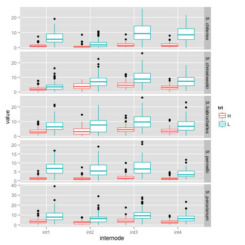
Q14
Create a boxplot for each combination of species, internode, and treatment.
pl <- ggplot(tom.melt, aes(x = internode, y = value, color = trt))
pl <- pl + geom_boxplot()
pl + facet_grid(species ~ ., scales = "free_y")
## Warning: Removed 12 rows containing non-finite values (stat_boxplot).
## Warning: Removed 23 rows containing non-finite values (stat_boxplot).
## Warning: Removed 8 rows containing non-finite values (stat_boxplot).
## Warning: Removed 43 rows containing non-finite values (stat_boxplot).
## Warning: Removed 22 rows containing non-finite values (stat_boxplot).
##Bonus: unmelt your data with cast If you include an indexing variable in your original data frame, you can use case to unmelt it.
tom.small$index <- 1:nrow(tom.small)
tom.melt2 <- melt(tom.small, measure.vars = 7:10)
head(tom.melt2)
##   shelf flat col row    acs trt ndvi     lat    lon  alt         species
## 1     Z    1   B   1 LA2580   H  111  -9.517 -78.01  740    S. pennellii
## 2     Z    1   C   1 LA1305   H  120 -13.383 -75.36 3360   S. peruvianum
## 3     Z    1   D   1 LA1973   H  110 -16.233 -71.70 2585   S. peruvianum
## 4     Z    1   E   1 LA2748   H  105 -20.483 -69.98 1020     S. chilense
## 5     Z    1   F   1 LA2931   H  106 -20.917 -69.07 2460     S. chilense
## 6     Z    1   G   1 LA1317   H  132 -13.417 -73.84 2000 S. chmielewskii
##   who index variable value
## 1 Dan     1     int1  2.37
## 2 Dan     2     int1  3.34
## 3 Dan     3     int1  8.43
## 4 Dan     4     int1  0.56
## 5 Dan     5     int1  0.82
## 6 Dan     6     int1  1.07
tom.small2 <- cast(tom.melt2)
tom.small2 <- tom.small2[order(tom.small2$index), ]
dim(tom.small)
## [1] 1008 17
dim(tom.small2)
## [1] 1008 17
head(tom.small)
##   shelf flat col row    acs trt int1 int2 int3 int4 ndvi     lat    lon
## 1     Z    1   B   1 LA2580   H 2.37 1.59 1.87 0.51  111  -9.517 -78.01
## 2     Z    1   C   1 LA1305   H 3.34 0.01 9.19 1.62  120 -13.383 -75.36
## 3     Z    1   D   1 LA1973   H 8.43 2.39 6.70 3.69  110 -16.233 -71.70
## 4     Z    1   E   1 LA2748   H 0.56 0.00 1.60 0.61  105 -20.483 -69.98
## 5     Z    1   F   1 LA2931   H 0.82 0.02 1.49 0.46  106 -20.917 -69.07
## 6     Z    1   G   1 LA1317   H 1.07 6.69 5.72 4.76  132 -13.417 -73.84
##    alt         species who index
## 1  740    S. pennellii Dan     1
## 2 3360   S. peruvianum Dan     2
## 3 2585   S. peruvianum Dan     3
## 4 1020     S. chilense Dan     4
## 5 2460     S. chilense Dan     5
## 6 2000 S. chmielewskii Dan     6
head(tom.small2)
##     shelf flat col row    acs trt ndvi     lat    lon  alt         species
## 815     Z    1   B   1 LA2580   H  111  -9.517 -78.01  740    S. pennellii
## 819     Z    1   C   1 LA1305   H  120 -13.383 -75.36 3360   S. peruvianum
## 823     Z    1   D   1 LA1973   H  110 -16.233 -71.70 2585   S. peruvianum
## 827     Z    1   E   1 LA2748   H  105 -20.483 -69.98 1020     S. chilense
## 831     Z    1   F   1 LA2931   H  106 -20.917 -69.07 2460     S. chilense
## 835     Z    1   G   1 LA1317   H  132 -13.417 -73.84 2000 S. chmielewskii
##     who index int1 int2 int3 int4
## 815 Dan     1 2.37 1.59 1.87 0.51
## 819 Dan     2 3.34 0.01 9.19 1.62
## 823 Dan     3 8.43 2.39 6.70 3.69
## 827 Dan     4 0.56 0.00 1.60 0.61
## 831 Dan     5 0.82 0.02 1.49 0.46
## 835 Dan     6 1.07 6.69 5.72 4.76
Posted by Julin Maloof