Prep
tomato <- read.table("TomatoR2CSHL.csv", header = T, sep = ",")
tomato <- na.omit(tomato)
library(ggplot2)
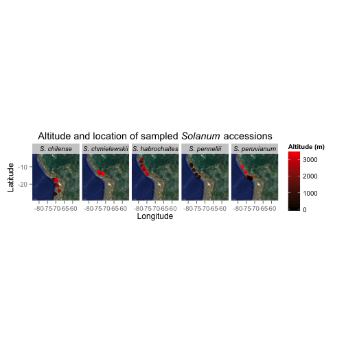
Kaisa
library(ggmap)
map <- get_map(location = c(lon = -70, lat = -16),
               zoom = 5,
               maptype = 'hybrid')
ggmap(map) +
  geom_point(aes(x      = lon,
                 y      = lat,
                 colour = alt),
             data       = tomato,
             size       = 2) +
             facet_grid(. ~ species) +
             scale_colour_continuous(   low  = "black",
                                        high = "red") +
             labs(  title = expression(paste("Altitude and location of sampled ", italic("Solanum"), " accessions")),
                        x = "Longitude",
                        y = "Latitude",
                   colour = "Altitude (m)") +
            theme( aspect.ratio = 1,
                   strip.text.x = element_text(face="italic"))
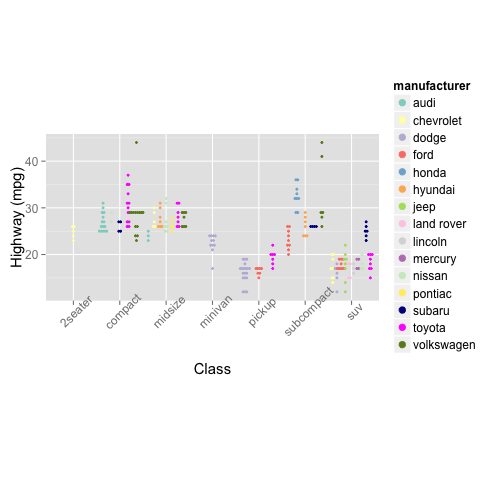
Stacey
library(RColorBrewer)
myColors <- c(brewer.pal(12, "Set3"), "#00008B", "#FF00FF", "#698B22")
colScale <- scale_colour_manual(name="manufacturer", values=myColors)
colScaleFill <- scale_fill_manual(name="manufacturer", values=myColors)
mpg.class <- ggplot(data=mpg, aes(x=class, y=hwy, fill=manufacturer, color=manufacturer))
mpg.class + geom_dotplot(binaxis="y", stackdir="center", dotsize=.8, position="dodge", binwidth=.5) + labs(x="Class", y="Highway (mpg)") +
  colScale + colScaleFill +
  theme(aspect.ratio=.5, text = element_text(size=15), axis.text.x = element_text(angle=45))
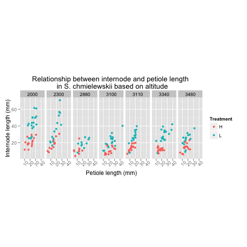
Amanda
I decided S. chmielewskii is my favorite species and wanted to explore the relationship between sun/shade internode and petiole length at different altitudes
data_chm <- subset(tomato, tomato$species=="S. chmielewskii")
data_chm$species <- factor(data_chm$species)
c_AS <- ggplot(data_chm, aes(petleng, intleng, colour=trt))
c_AS <- c_AS + geom_point() +
                facet_grid(.~alt) +
                ggtitle("Relationship between internode and petiole length \n in S. chmielewskii based on altitude") +
                xlab("Petiole length (mm)") +
                ylab("Internode length (mm)") +
                labs(color = "Treatment") +
                theme(aspect.ratio = 2.5,
                    axis.text.x  = element_text(angle = 45))
c_AS
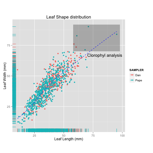
Miguel
p<-ggplot(tomato, aes(x      = leafleng,
                   y      = leafwid,
                   colour = who))
p +geom_point() +
  geom_rug() +
  labs(x = "Leaf Length (mm)",
       y = "Leaf Width (mm)",
       title="Leaf Shape distribution",
       colour="SAMPLER") +
  theme(aspect.ratio = 1)+
  annotate("rect",xmin=58, xmax=98,ymin=70, ymax=92, alpha=0.3)+
  annotate("text", x=85, y=67, label="Clorophyl analysis")+
  geom_smooth(se=FALSE, colour="blue", linetype=2 )
Palmer
Goal: to make better for old people with failing eyes and colorblindness, increase point size, change shape and color, remove gray background, increase font, bold font, add fit lines
cbbPalette <- c("#000000", "#E69F00", "#56B4E9", "#009E73", "#F0E442", "#0072B2", "#D55E00", "#CC79A7")
ggplot(tomato, aes(x= leafleng,
                   y= leafwid,
                   colour = who, shape=who)) +
  theme_bw() +
  theme(panel.grid.major = element_line(colour = "black", size=2))+
  theme(panel.border = element_rect(colour = "black", size =2)) +
  geom_point(size=3) +
  geom_rug() +
  labs(x = "Leaf Length (mm)",
       y = "Leaf Width (mm)") +
  theme(axis.title.x = element_text(face="bold", colour="black", size=20),
        axis.text.x  = element_text(angle=90, colour="black", vjust=0.5, size=16)) +
  theme(axis.title.y = element_text(face="bold", colour="black", size=20),
      axis.text.y  = element_text(angle=0, colour="black", vjust=0.5, size=16))+
  theme(legend.title = element_text(colour="black", size=16, face="bold")) +
theme(legend.text = element_text(colour="black", size=16, face="bold")) +
  geom_smooth(method=lm, size=2) +
  scale_fill_manual(values=cbbPalette)+
scale_colour_manual(values=cbbPalette)+
  theme(aspect.ratio = 1)
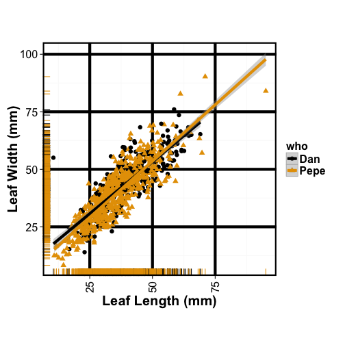
After, it’s less lovely but more visible!
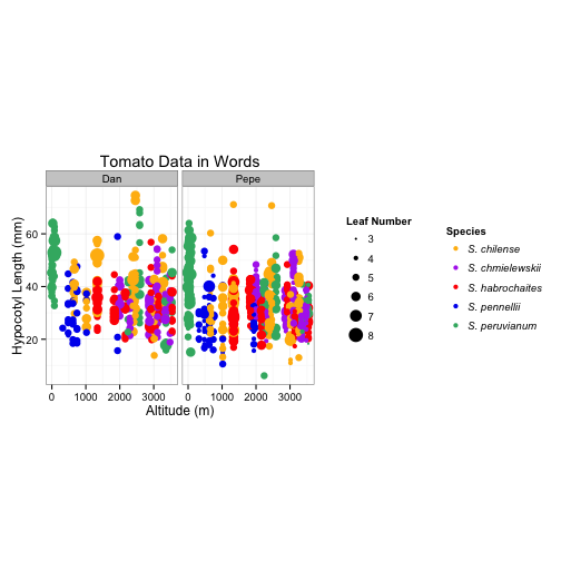
Jessica
library(gridExtra)
library(gtable)
#1 draw a plot with the leaf number legend
plot1 <-  ggplot(tomato) +
        geom_point(aes(alt, hyp,
                   size  = leafnum)) +
    labs( size = "Leaf Number" ) +
    theme_bw(base_size = 12, base_family = "") +
    theme (legend.key = element_rect(colour = "white"))
# Extract the leaf number legend - leg1
leg1 <- gtable_filter(ggplot_gtable(ggplot_build(plot1)), "guide-box")
#2 draw a plot with the species legend
# List of colors http://www.stat.columbia.edu/~tzheng/files/Rcolor.pdf
plot2 <-  ggplot(tomato) +
    geom_point(aes(alt, hyp,
                   color = species)) +
    labs( color = "Species" ) +
    theme_bw(base_size = 12, base_family = "") +
    theme (legend.key = element_rect(colour = "white"),
           legend.text = element_text( face = "italic")) +
    scale_colour_manual(values = c("darkgoldenrod1", "darkorchid2", "red","blue2", "mediumseagreen"))
# Extract the species legend - leg2
leg2 <- gtable_filter(ggplot_gtable(ggplot_build(plot2)), "guide-box")
# Draw a plot with no legends - plot
plotNoLegends <-  ggplot(tomato) +
  geom_point(aes(alt, hyp,
                   size  = leafnum,
                   color = species)) +
  facet_grid(. ~ who) +
  theme_bw(base_size = 12, base_family = "") +
  theme (aspect.ratio = 1.5,
         legend.position = "none") +
  labs(title = "Tomato Data in Words",
       x     = "Altitude (m)",
       y     = "Hypocotyl Length (mm)") +
   scale_colour_manual(values = c("darkgoldenrod1", "darkorchid2", "red","blue2", "mediumseagreen"))
#If I use this it puts the legends side by side
plotAllTogether <- arrangeGrob(plotNoLegends, leg1,
          widths = unit.c(unit(1, "npc") - leg1$width, leg1$width), nrow = 1)
plotAllTogether <- arrangeGrob(plotAllTogether, leg2,
          widths = unit.c(unit(1, "npc") - leg2$width, leg2$width), nrow = 1)
grid.newpage()
grid.draw(plotAllTogether)
# Now I want to try to get them stacked
grid.arrange(plotNoLegends, arrangeGrob(leg1, leg2, ncol=1),
                    ncol=2, widths=c(1.5,0.5))
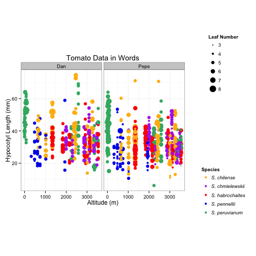
# Well now they are stacked but they are spaced a little far apart for my taste, but I
# cannot figure out how to get them spaced closer together.
Hsin-Yen
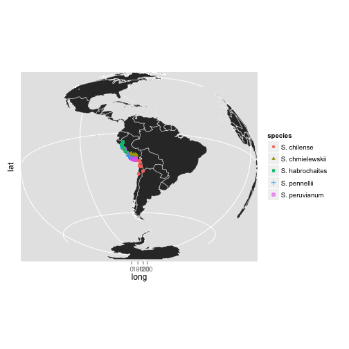
library(maps)
world = map_data("world")
MAP = ggplot(world, aes(long, lat),group=group)
Polygon = geom_polygon(aes(group = group), colour="white",size=0.2)
Points = geom_point(data=tomato,aes(lon, lat, shape=species, colour=species),size=2)
Theme = theme(aspect.ratio=0.8)
MAP+Polygon+Theme+Points+coord_map("ortho", orientation=c(-21, -70, 0))
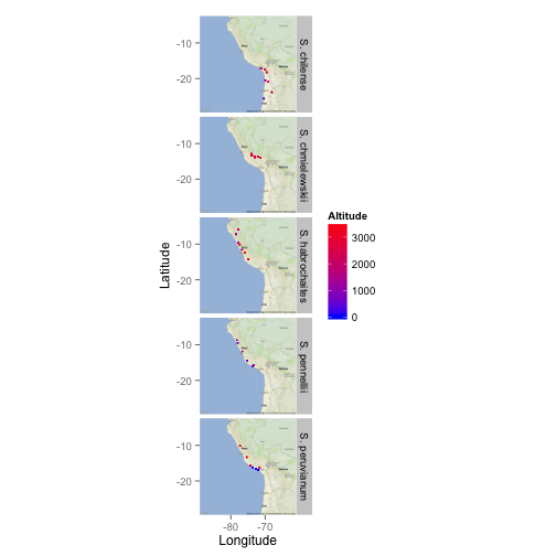
Polly
library(ggmap)
map <- get_map(location = c(lon = -75, lat = -16), zoom     = 5,
              maptype  = 'roadmap' )
ggmap(map) +
 geom_point(aes(x = lon, y = lat, colour = alt), data = tomato, size = 0.6) +
 facet_grid(species ~ .) +
 scale_colour_continuous(low  = "blue", high = "red") +
 labs(x = "Longitude", y ="Latitude", colour = "Altitude")
Moran
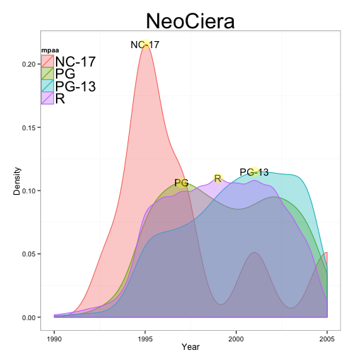
#Optimized Ciera
submovies <- subset(movies, mpaa !="" & year>=1990)
ciera <- ggplot(submovies, aes(year,
                              fill = mpaa,
                              colour = mpaa))+
  geom_density(name= "MPAA", alpha  = 0.35)
#neo
neoceira <- ciera+
  ylab("Density")+
  xlab("Year")+
  labs(title = 'NeoCiera')+
  theme_bw()+
  theme(aspect.ratio = 1,
        legend.position = c(.1,.85),
        legend.background = element_blank(),
        panel.grid.major = element_blank(),
        legend.text = element_text(size = 20),
        plot.title = element_text(size = 30)
  )
#more
r = subset(submovies, mpaa=="R")
rD = density(r$year)
rDy = rD$y
rDm = subset(rDy, rDy == max(rDy))
#
nc = subset(submovies, mpaa=="NC-17")
ncD = density(nc$year)
ncDy = ncD$y
ncDm = subset(ncDy, ncDy == max(ncDy))
#
pg = subset(submovies, mpaa=="PG")
pgD = density(pg$year)
pgDy = pgD$y
pgDm = subset(pgDy, pgDy == max(pgDy))
#
pg13 = subset(submovies, mpaa=="PG-13")
pg13D = density(pg13$year)
pg13Dy = pg13D$y
pg13Dm = subset(pg13Dy, pg13Dy == max(pg13Dy))
#
y = c(rDm, ncDm, pgDm, pg13Dm)
x = c(1999, 1995, 1997, 2001)
label = c("R", "NC-17", "PG", "PG-13")
#
neoceira + annotate('text', x=x, y=y, label = label)+
  annotate('point', x=x, y=y, label=label,
           size = 7, colour = 'yellow', alpha =0.35)
Cody
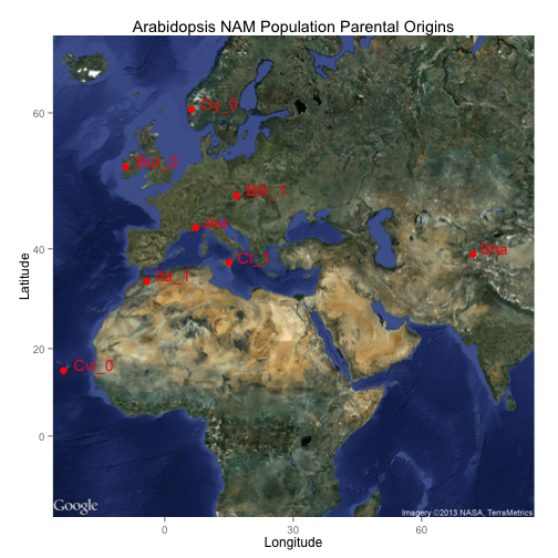
library(ggmap)
NAM <- read.csv("NAM_lat_long_data.csv")
head(NAM)
##   Ecotype_name           Location   lat    long
## 1          Jea             France 43.68   7.333
## 2        Ita_1            Morocco 34.00  -4.200
## 3         Ct_1              Italy 37.52  15.067
## 4        Cvi_0 Cape_verdi_islands 15.11 -23.617
## 5        Bur_0            Ireland 53.05  -9.100
## 6        Blh_1     Czechoslovakia 48.83  16.749
nam_map <- get_map(location= c(lon = 30, lat = 35),
                zoom=3,
               maptype = 'satellite')
ggmap(nam_map) +
geom_point(colour='red', size= 3, aes(x=long, y=lat), data=NAM) +
geom_text(data = NAM, aes(x = long, y = lat, label = Ecotype_name),
          size = 5, vjust = 0, hjust = -0.25, colour='red') +
theme(aspect.ratio = 1) +
labs(title="Arabidopsis NAM Population Parental Origins",
            x="Longitude", y="Latitude")
Upendra
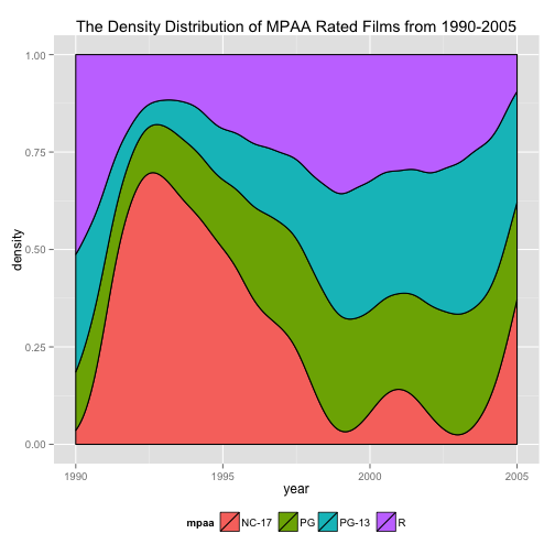
# Figure 2:
movies_new<-subset(movies, mpaa!="" & year>=1990)
ggplot(movies_new, aes(year, fill = mpaa)) + stat_density(aes(y = ..density..), position = "fill", color = "black") + xlim(1990, 2005) + theme(legend.position = "bottom") + labs(title = "The Density Distribution of MPAA Rated Films from 1990-2005")
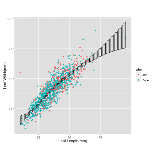
# Figure 4:
ggplot(tomato, aes(leafleng, leafwid)) + geom_point(aes(colour = who)) + theme(aspect.ratio = 1) + labs(x="Leaf Length(mm)", y="Leaf Width(mm)") + stat_smooth(geom = "errorbar")
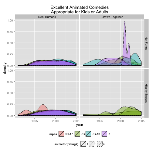
Donnelly
mymov3 <- subset(x=movies, year>1990 & mpaa !="")
mymov3$Comedy2 <- factor(mymov3$Comedy, labels = c("Not Funny", "Hilarity Ensues"))
mymov3$Animation2 <- factor(mymov3$Animation, labels = c("Real Humans", "Drawn Together"))
mymov3$rating2 <- round(mymov3$rating)
mymov3$rating2 <- c(1, 3, 4)
ggplot(data = mymov3, mapping = aes( x = year,  fill = mpaa, linetype = as.factor(rating2) ) ) +
  geom_density(alpha=0.4) +
  labs(title="Excellent Animated Comedies\nAppropriate for Kids or Adults" ) +
  theme(legend.position = "bottom") +
  facet_grid(Comedy2~Animation2)